Modelling
Mathematical methods can be used to calculate the continuous spatial concentration distribution of pollutants and its change over time, if we know the properties of atmospheric flows and individual pollutants, the location of the most important pollutant sources, and their outputs. In addition, mathematical models describing the distribution and transformation of pollutants, combined with meteorological forecasting models, provide an opportunity to estimate the expected evolution of air pollution.
Similarly to weather forecasting, air quality forecasting relies on complex mathematical models which describe the physical and chemical processes that take place in the atmosphere using the tools of mathematics. The predicted concentration values determined by the forecasting model system is significantly influenced by the meteorological conditions. The quality of the prediction of the wind direction and velocity, the spatial distribution and amount of precipitation, and the height of the mixing layer influence the accuracy of the forecast of concentration fields. Accurate knowledge of the temporal and spatial variability of the gridded emission data is also a significant factor which influence the accuracy of the air quality forecast. For these reasons, the prediction may be inaccurate, and sometimes there could be significant differences between the measured and predicted concentration values.
The model system is based on the CHIMERE chemical transport model. The input meteorological data required for the model-system are provided by the AROME fine-resolution numerical weather prediction model. The input gridded emission database, which is also crucial for the model simulation, consists of data for 2015. The model takes into account chemical transformations in the atmosphere, describes more than 300 reactions of 80 gaseous species. The spatial resolution of the calculations for the Hungarian area is approximately 10 km, which means that the calculated values are average values for an area of 10x10 km. It has to be noted that this type of model is not able to take into account local effects (e.g. direct effect of high-traffic roads within a few hundred meters).
Forecast Maps
For the visualization of the different air pollutant concentration forecasts on maps, we used the European Air Quality Index (EAQI) categories/colours defined by the European Environment Agency (EEA). In contrast to the original definition of the air quality index which says that the visualized colour belongs always to the pollutant, which has the highest value at the moment compared to the allowed threshold limit (meaning that it is the worst from an air quality point of view), we coloured the forecast maps separately, following the EAQI.
EPSgram (Probabilistic forecast)
Every forecast model aims to describe correctly the main physical processes taking place in the atmosphere. These physical processes are very difficult to describe using mathematics, so some simplifications are needed. However, these simplifications inevitably introduce errors into the forecasts. To get an idea of these errors, we used the multi-model ensemble method. The output of several different chemical transport models is used to produce the so-called meteogram, or EPSgram, which shows the limits within which the predicted concentration values vary and indicates which prediction is the most likely to occur based on the models' calculations.
The EPSgrams presented on our website are created using the results of the 11 chemical transport models of the CAMS (Copernicus Atmosphere Monitoring Service) Regional system.
PBL (planetary boundary layer) height
The planetary boundary layer (PBL) is the lowest part of the troposphere that is influenced by the earth's surface. It responds to physical impacts on a time scale of up to an hour. Examples of physical effects are friction, evaporation and transpiration, heat transfer, pollutant emissions, surface-induced changes in the flow field. The thickness of the PBL typically ranges from a few hundred meters to a few kilometres, depending, for example, on the time of year, time of day, and latitude. So it is a function of both space and time. The height of the PBL shows a marked diurnal cycle, which is related to the incoming solar radiation. The soil surface absorbs most of the radiation during the day, so it heats up and warms the lowest part of the atmosphere. These lower air masses have become warmer than their surroundings, so they are starting to rise. Due to the convective movements thus formed, the thickness of the PBL increases. So the surface has an effect on the evolution of the PBL. Atmospheric materials are transported within the PBL by transport processes. Horizontal transport (i.e. advection) is controlled by the wind, which average speed is between 2 and 10 m / s in the PBL. The wind speed is lowest in the layers closest to the surface due to friction and typically increases upwards. The air movement in the vertical direction is less strong than in the horizontal one. Its speed is a few mm/s or cm/s. Turbulence is one of the most important transport processes, it is also involved in the intensive mixing of the air. Sometimes the PBL is defined by turbulent processes.
PBL plays an important role in air quality, as most atmospheric pollutants are distributed in this layer. The more accurately we know the characteristics of the PBL and the processes that take place here, the more precisely we can describe and monitor the evolution of air pollution.
SI (Stagnation index)
SI is a measure of the atmosphere's ability to dilute air pollutants. Stagnant air allows pollutants to accumulate in a given area. This is often caused by an anticyclone, temperature inversion, or low wind speed. The value of SI shows a positive correlation with the values of both ground-level ozone and PM10 concentration. The maps show the spatial and temporal changes in the value of the SI index. Shades of red on the maps show where meteorological conditions are favourable to the accumulation of pollutants, thus air quality in these areas is expected to deteriorate.
Aerosol Optical Depth (AOD)
Aerosol Optical Depth (AOD) is a measure of the total amount of aerosol particles in an atmospheric column. These particles, which can be solid or liquid, are suspended in the air and come from both natural sources like volcanic ash, sea salt spray, and desert dust, as well as from human activities, including the burning of fossil fuels and vegetation, which produce soot and smoke. Aerosol particles scatter and diffuse sunlight, and the extent of this radiative effect is captured by AOD. In addition to tracking standard air pollutants, CAMS also offers global forecasts of AOD trends. On our website, we provide visualizations of total aerosol content, as well as the radiative forcing of five specific components—sea salt, dust, biomass burning, black carbon, and sulphate—using modelled CAMS AOD data.
Related articles from modelling category